Hadley Cells
Farrell's theory about the extension of the Hadley Cells has a mathematical basis, and he argues his case through the derivation of atmospheric dynamics equations. He starts with an overview of the work done in Held and Hou (1980) and then modifies the equations to account for his ideas. In a similar manner, the following information will walk through the work done by Held and Hou and then will present the modified equations derived by Farrell. These steps follow sections 11.2 and 11.3 in Atmospheric and Oceanic Fluid Dynamics by Geoffrey K. Vallis (2006).
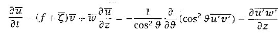
For the model of the Hadley circulation, the atmosphere is assumed to be a Boussinesq atmosphere. As a result, the zonally averaged momentum equation in the absence of friction is
 (1)
(1)
The overbars represent zonal averages. If vertical advection is considered to be small in comparison to horizontal advection and if we ignore the eddy terms on the right-hand side of the equation, then a steady state solution is
![]() (2)
(2)
If we assume that meridional flow is not zero, then f + ζ = 0. Another way of writing this equation is
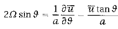 (3)
(3)
where the left side equals f and the right side equals ζ. We assume that the zonal flow at the equator is zero because air rises from the surface there where the flow is weak by assumption. A solution to equation 3 is then
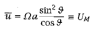 (4)
(4)
This equation provides the zonal velocity of a particle moving toward the poles in the upper part of the circulation. We can also derive this equation from the conservation of angular momentum, m, of an air parcel at certain latitude ϑ. Angular momentum can be represented as
![]() (5)
(5)
If zonal velocity equals zero at the equator and if a polewards moving air parcel conserves momentum, equation 5 leads directly to equation 4. Also taking the derivative of equation 5 with respect to latitude reveals
 (6)
(6)
These steps demonstrate that if friction and eddy fluxes can be ignored, then air moving towards the pole in the Hadley Cell will conserve its angular momentum. This fact means that an air parcel moving polewards must accelerate zonally as it moves toward the high-latitudes, so the zonal velocity will increase with latitude.
Since the zonal velocity is assumed to be low near the surface and since equation 4 provides the zonal velocity in the upper branch of the Hadley Cell, an estimate for the velocity gradient over the height of the cell is known. This fact means that we can use the thermal wind equation to find the vertically averaged temperature. While the geostrophic wind relation does not hold at the equator, it is accurate until very close to the equator. Therefore, the traditional thermal wind equation works for the model. This equation is
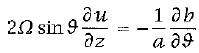 (7)
(7)
"where b = g δθ/θ0 is the buoyancy and δθ is the deviation of potential temperature from a constant reference value θ0" (Vallis 460). Substituting in equation 4 for u and vertically integrating the equation from the ground to a height H provides
 (8)
(8)
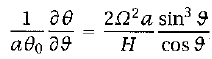
where θ = H-1* ∫H0δθ dz is the vertically averaged potential temperature. Assuming that the latitudinal extent of the Hadley Cell is not too great, we can use the small angle approximation and can replace sin ϑ with ϑ and cos ϑ with 1. After then integrating equation 8, it becomes
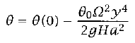 (9)
(9)
where y = aϑ and θ(0) is the potential temperature at the equator. The value of this term is still unknown at this point, so we must use thermodynamics to obtain it. For this model, we will assume "that the thermodynamic forcing can be represented by a Newtonian cooling to some specified radiative equilibrium temperature, θE" even though this assumption is a big simplification (Vallis 460). The thermodynamic equation we shall use is
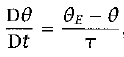 (10)
(10)
where τ is a relaxation time scale. If we assume that the radiative equilibrium temperature falls from the equator to the pole and that it increases with height, a simple equation for it is
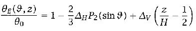 (11)
(11)
"where ΔH and ΔV are non-dimensional constants that determine the fractional temperature difference between the equator and the pole and [between] the ground and the top of the fluid, respectively" (Vallis 460). P2 is the second Legendre polynomial and is often the leading term in the Taylor expansion of symmetric functions around the equator. P2(y) = (3y2 - 1)/2. With the small angle approximation and at z = H/2, equation 11 becomes
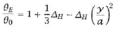 (12)
(12)
or
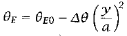 (13)
(13)
"where θE0 is the equilibrium temperature at the equator, Δθ determines the equator-pole-radiative equilibrium temperature difference, and" (Vallis 461)
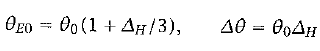 (14)
(14)
If we assume that equation 9 is valid between the equator and some latitude ϑH where the meridional velocity is zero, we create a closed system between the equator and this latitude. To conserve potential temperature, the solution to equation 9 must uphold
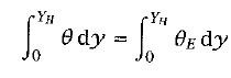 (15)
(15)
where YH = aϑH. This requirement creates a closed system in which heat flows from the equator to ϑH to balance the atmosphere's natural heating and cooling by absorption and emission of heat. A second constraint is that the solution must be continuous at y = YH, meaning
![]() (16)
(16)
Plugging equations 9 and and 13 into equations 15 and 16 yield
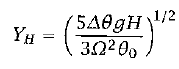 (17)
(17)
and
 (18)
(18)
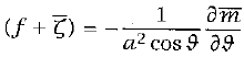
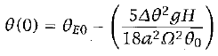
These final equations reveal that the Hadley Cell should have a finite meridional extent. Held and Hou reached this conclusion for an inviscid atmosphere (1980), and their work agrees with the dynamics seen in the real atmosphere. Farrell uses this work as a starting point for his idea, but he modifies the equations to include friction. Instead of fully walking through all of his steps, which are similar to those of Held and Hou, the final equations that Farrell reaches are
In these equations, R stands for the Rossby wave number, and Γ represents "a measure of the relative dominance of the radiation and momentum time scales" and can be thought of as a friction term (Farrell, 1990). R = gHϑ/ω2 a2, and Γ = SτR/ϑhτ v. These equations have a solution with a Hadley Cell beginning at the equator where Vb(0) = 0 and ending at the poles where Vb (yH) = 0. R and Γ determine this solution and, thus, are important factors for the Hadley Cell circulation.
As mentioned before, the height of the tropopause has a significant impact on the extent of the Hadley Cells. Looking at Farrell's equations, one can now see how this fact is true. The height, H, is influential in determining the value of the Rossby wave number. If the height doubles, the Rossby wave number will also double. Using the first of Farrell's equations, one can see that an increase in the Rossby wave number will decrease the change in potential temperature over latitude. This change will cause the temperature gradient to decrease throughout the extent of the Hadley Cell. Since the Hadley Cells extend as the Rossby wave number increases, the Hadley Cells will extend to the poles if R increases enough, and thus, the EPTD will decrease significantly.
Similarly, Γ plays an important role in atmospheric dynamics. It is important to note that the amount by which a torque will decrease angular momentum depends on the mass flux Vb, which is determined by SτR, which is part of Γ. In an inviscid atmosphere, Γ is set to zero, but in an atmosphere with friction, it must have a non-zero value. Since Γ determines how much a torque will decrease angular momentum, the zonal velocity decreases as Γ increases. Therefore, if Γ increases substantially, a large enough torque could be generated to prevent the formation of a zonal wind strong enough to stop an air parcel from moving poleward. As a result, a large Γ value could enable the Hadley Cells to extend all the way to the poles. This change would allow warm air from the equator to reach the high-latitudes and would reduce the EPTD to levels seen during equable climates.
Therefore, one can see that R and Γ are highly influential on the extent of the Hadley Cells. If both parameters increased enough during the Cretaceous and the Eocene, the Hadley Cells could have extended all the way to the poles. Under these conditions, air from the equator would have traveled all the way to the high-latitudes and would have heated the poles enough to have caused the equable climates.